Just two days ago, Desmos added a new feature to its graphing calculator to include support for complex numbers. In this post, I want to briefly share how to graph a Newton fractal in Desmos. This kind of process also applies to any fractal generated by applying an iterated function on the complex plane, such as the Mandelbrot set.
Using Complex Mode
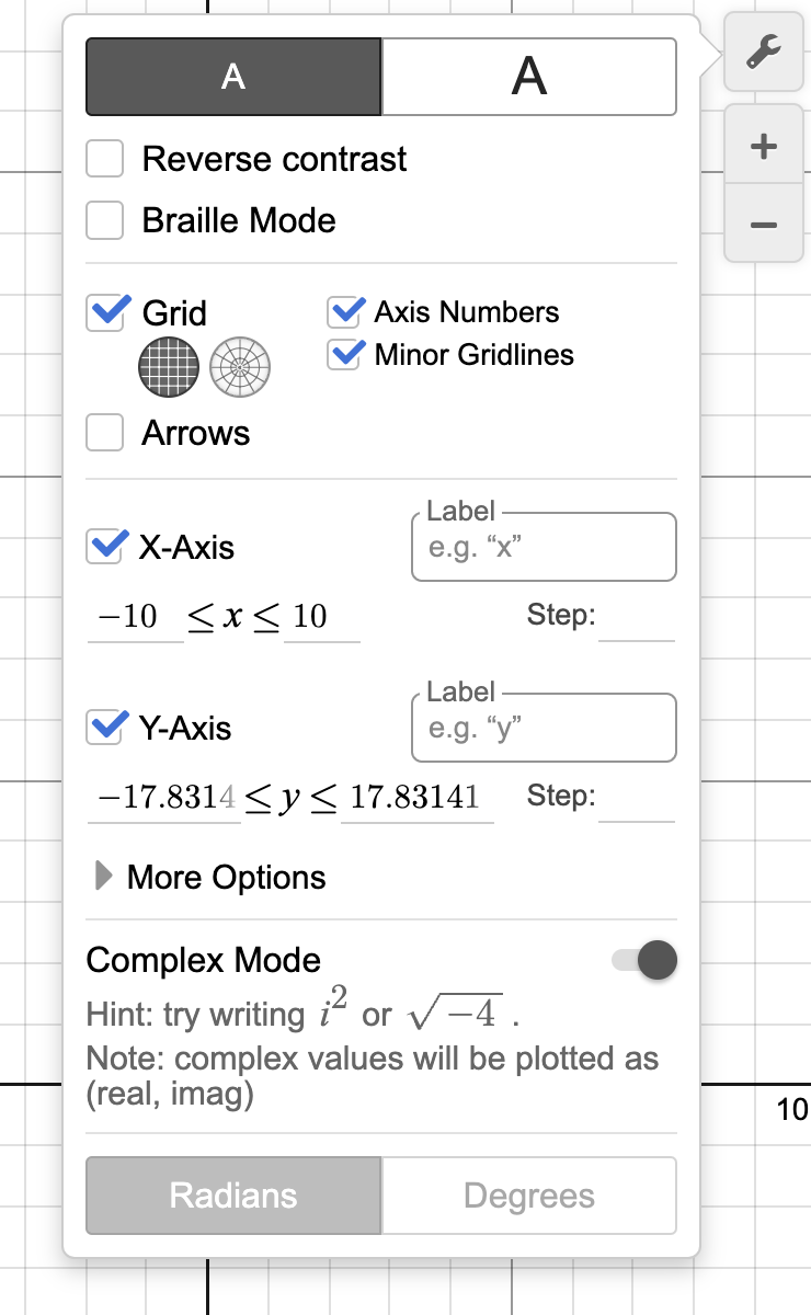
To use Complex Mode, you simply need to click on the wrench icon and enable it near the bottom of the settings panel.
Newton’s Method
Newton’s method (or the “Newton-Raphson method”) is a ubiquitous root-finding method. It is useful in many cases where you would like to find when an input to a function makes the function’s output 0, especially when that question is difficult or impossible to solve exactly. Newton’s method begins with an initial guess that is already near a root where the function of interest is locally similar to a linear function (I’ll elaborate on what this means), and it “iterates” to get a progressively closer and closer approximation of a root. However, interesting fractal properties emerge when you observe how the solutions that it converges to change with different initial guesses that are far from the root.
Newton’s method begins with a polynomial, \(p\left(z\right)\in\mathbb{C}\left[z\right]\), of which we would like to find the root (the value of \(x\) for which \(p\left(x\right)=0\)). Here, I will use the prototypical example function used to plot a Newton fractal:
$$p\left(z\right)=z^{3}-1$$
Newton’s method is essentially to use the function value and the derivative of the function at a current guess of the root to find a more accurate guess for the root. If the function can be approximated well near the guess using a linear function, then the root of that approximating linear function (which is very easy to find) is likely to be a good guess for the root of the actual function. When this is done repeatedly, the guess will typically converge to the root.
You can see this if you Taylor expand the function \(f\left(x\right)\) about the guess \(x_{n}\):
$$f\left(x\right)=f\left(x_{n}\right)+f’\left(x_{n}\right)\left(x-x_{n}\right)+\frac{1}{2}f’’\left(x_{n}\right)\left(x-x_{n}\right)^{2}\cdots$$
\(\left(x-x_{n}\right)\) gets very close to zero in the limit as \(x_{n}\) approaches \(x\), and so higher-order terms like \(\left(x-x_{n}\right)^{2}\) and \(\left(x-x_{n}\right)^{3}\) have much smaller contributions to the function value than the linear and constant terms of the expansion. These two terms create our linear approximation of the function:
$$f\left(x\right)\approx f\left(x_{n}\right)+f’\left(x_{n}\right)\left(x-x_{n}\right)$$
Geometrically, you construct a tangent line on the function at the current guess, and the point where it intersects the x-axis is the new revised guess. You then repeat this until you reach a desired accuracy.
We can solve for the linear approximation’s root exactly:
$$f\left(x\right)\approx f\left(x_{n}\right)+f’\left(x_{n}\right)\left(x-x_{n}\right)=0$$ $$f’\left(x_{n}\right)\left(x-x_{n}\right)=-f\left(x_{n}\right)$$ $$x-x_{n}=-\frac{f\left(x_{n}\right)}{f’\left(x_{n}\right)}$$ $$x=x_{n}-\frac{f\left(x_{n}\right)}{f’\left(x_{n}\right)}$$
Now we can repeatedly apply this calculation, where the approximate \(x\) that we compute becomes the new \(x_n\) for the next iteration.
Newton Fractals
Mathematically, Newton’s method repeatedly applies the fixed-point iteration
$$z\mapsto z-\frac{p\left(z\right)}{p’\left(z\right)}$$
Which, in this example, is
$$z\mapsto z-\frac{z^{3}-1}{3z^{2}}=\frac{1}{3z^{2}}+\frac{2z}{3}$$
Since this iteration is very simple, I decided to nest two iterations into one (so that I wouldn’t have to nest the function as many times). I.e., we define
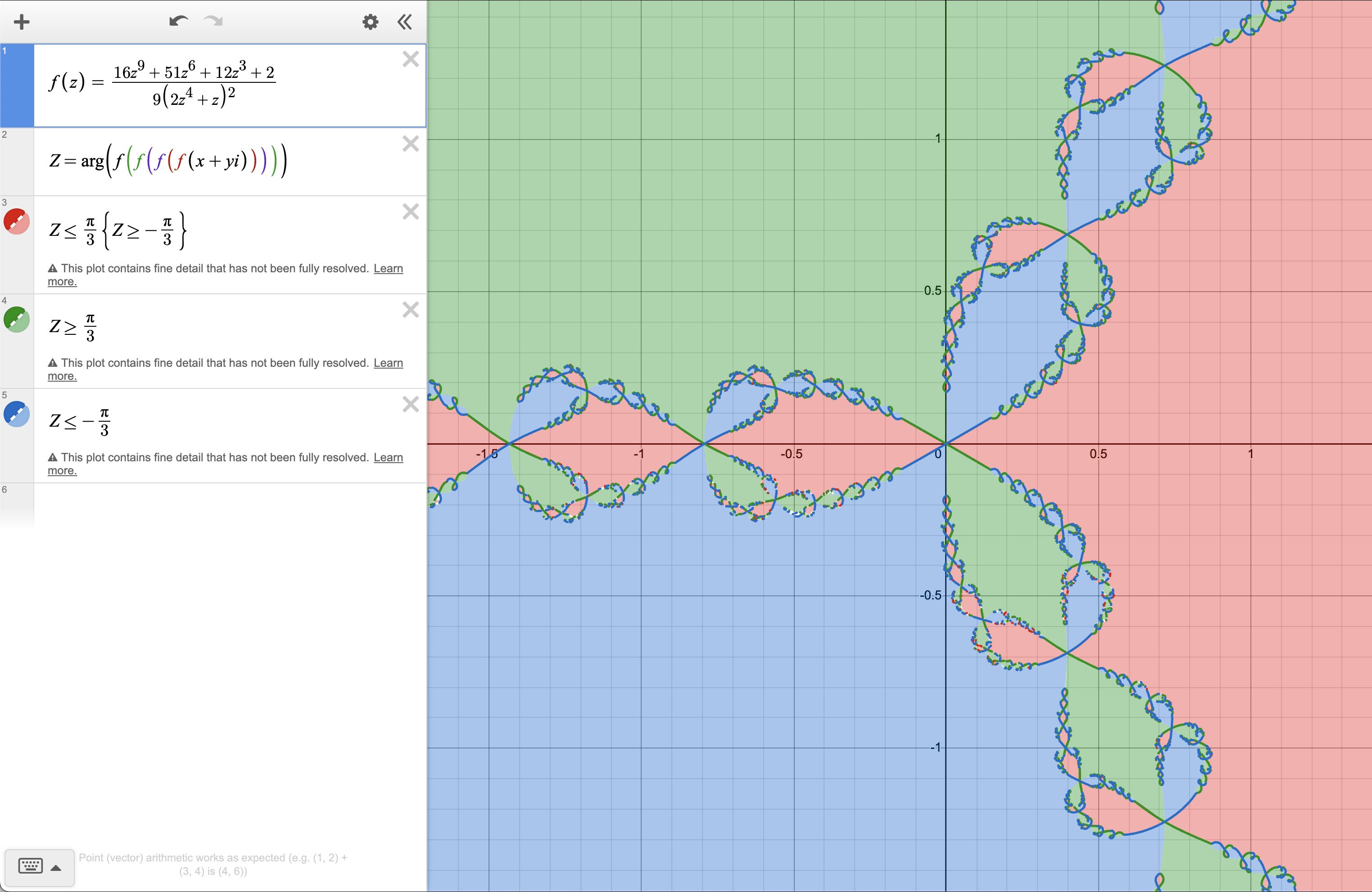
$$z\mapsto \frac{1}{3\left[\frac{1}{3z^{2}}+\frac{2z}{3}\right]^{2}}+\frac{2\left[\frac{1}{3z^{2}}+\frac{2z}{3}\right]}{3}$$ $$=\frac{16z^{9}+51z^{6}+12z^{3}+2}{9\left(2z^{4}+z\right)^{2}}$$
This method does a good job finding a complex root of the polynomial \(p\left(z\right)=z^{3}-1\) with quadratic convergence when we initialize with a decent approximation of the root. However, a fractal arises when we consider which root the function converges to when our initial value is far from any of the roots. The typical method of coloring the Newton fractal is to color each point on the complex plane a color based on which root that point would converge to when the iteration function is applied an infinite number of times. Since we can’t really apply the function an infinite number of times, we simply apply it many times and check which root the final point is closest to, as an approximation. To find which root the approximation is closest to, we only need to check the argument of the approximation, since this simple example has the 3rd roots of unity as solutions. Due to the new update, programming this in Desmos is relatively straight-forward: