Introduction
In this blog post, I derive two efficient methods to stably compute the infinite tetration (or “power tower”). “Tetration” simply means repeated exponentiation, so “infinite tetration” simply means exponentiation an infinite number of times. The infinite tetration of \(x\), which I will call \(y\), is defined as:
\[y=x^{x^{x^{.^{.^{.}}}}}\]
I will begin with a simple “naïve” approach to solving the problem. Then, I will more deeply analyze the structure of the problem. From there, I will discuss two approaches to solving the problem efficiently.
The first method I derive turns the problem into an integral which can be solved numerically. The second method that I derive, and the main focus of this blog post, is an iterative method that achieves stable quadratic convergence for all valid \(x\). “Iterative” simply means that the method constructs successively more accurate approximations until the approximation error is within a desired tolerance of the true solution.
The Naïve Approach
The most straightforward way to compute the infinite power tower \(y\) of an input \(x\) is to repeatedly raise \(x\) to the power of more \(x\)’s. The idea is that the infinite power tower, which we can not compute (it requires an infinite number of operations), is sufficiently similar to a very large power tower, which we can compute. As we will discover later, however, there are certain inputs where this approach is problematic. It is important to note that repeated exponentiation is right-associative, not left-associative. That means \(a^{b^{c}}=a^{\left(b^{c}\right)}\neq\left(a^{b}\right)^{c}\). Mathematically, the Naïve approach is then:
\[y_0 = x\] \[y_1 = x^x = x^{y_0}\] \[y_2 = x^{x^{x}} = x^{y_1}\] \[\vdots\] \[y_n = x^{y_{n-1}}\]
In the limit as we raise \(x\) to the power of itself more times, it converges on the solution \(y\) if one exists. However, this approach converges quite slowly for many values of \(x\). Furthermore, for small \(x\), the sequence oscillates indefinitely, and the values between which it oscillates converge.
To see how inefficient this is for some inputs, look at this example of convergence of 0.4 raised to the power of itself repeatedly:
| n | \(y_n\) | Absolute error ( \(\left | y_n-y_{\infty}\right | \) ) |
|---|---|---|
| 0 | 0.40000000000 | 0.18504317197 |
| 1 | 0.69314484316 | 0.10810167118 |
| 2 | 0.52987073647 | 0.05517243550 |
| 3 | 0.61537979747 | 0.03033662550 |
| 4 | 0.56900457469 | 0.01603859728 |
| 5 | 0.59370446436 | 0.00866129238 |
| … | … | … |
| 35 | 0.58504317204 | 0.00000000007 |
| 36 | 0.58504317194 | 0.00000000003 |
| 37 | 0.58504317199 | 0.00000000002 |
| 38 | 0.58504317196 | 0.00000000001 |
| 39 | 0.58504317198 | 0.00000000001 |
Here is an example of “oscillatory” behavior with 0.02 raised to the power of itself repeatedly:
| n | \(y_n\) |
|---|---|
| 0 | 0.0200000000 |
| 1 | 0.9247420362 |
| 2 | 0.0268467067 |
| 3 | 0.9003020739 |
| … | … |
| 26 | 0.0314614034 |
| 27 | 0.8841949279 |
| 28 | 0.0314614938 |
| 29 | 0.8841946152 |
| 30 | 0.0314615323 |
As we approach an infinite number of iterations, the sequence tends toward bouncing between two values. Of course, you might imagine that large numbers raised to the power of themselves will keep getting larger forever. Here is an example of 1.5 raised to itself repeatedly, where the infinite tetration spirals to infinity:
| n | \(y_n\) |
|---|---|
| 1 | 1.500000000 |
| 2 | 1.837117307 |
| 3 | 2.106203352 |
| … | … |
| 9 | 4.382546732 |
| 10 | 5.911914873 |
| 11 | 10.99098293 |
| 12 | 86.18189174 |
| 13 | 1,499,263,005,586,587 |
| 14 | 5.400339825 × 10^264,007,110,309,345 |
By the 14th iteration, it is quite evident that the sequence tends to infinity.
To better understand these types of behaviors, I’ve plotted the true infinite tetration curve below, in green, alongside the naïve approach for computing it, in red:
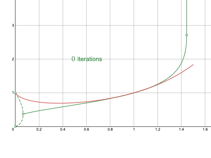
Notice how, for small values below a threshold between 0 and 0.2, the numbers oscillate between two values in the limit as the number of iterations approaches infinity. These two values are denoted by the dashed green line. In this region, the infinite tetration is technically not defined, because it does not converge to a single value. Above that “branching point,” until a point a bit greater than 1.4, the infinite tetration does converge to a single value. These are denoted by the solid green line. Finally, above some point between 1.4 and 1.5, the infinite tetration diverges toward infinity.
Given these observations, I would like to answer the following questions:
- When does the infinite tetration converge? When does it oscillate indefinitely? When does it blow up to infinity? Can we rigorously derive exactly where these transitions occur?
- Can we find a “better” way to compute the result of the infinite tetration (either what value the sequence converges to, or between what values it oscillates between)?
Moving forward in this blog post, I will neglect the infinite tetration of negative numbers. This is because, inevitably, you will encounter complex numbers; I wish to remain within the reals this time. The only exception to this is the infinite tetration of -1, which is -1. And that’s rather boring.
In the next section, Structure Analysis, I will address the first bullet point. In the following two sections, Lambert W and Newton-Raphson, I will address the second bullet point.
Structure Analysis
Fixed-Point Iteration
Recall the naïve approach:
\[y_n = x^{y_{n-1}}\]
We say that the sequence “converges” if the limit \(y_{\infty}=\lim_{n\to\infty}y_n\) exists. If the sequence does indeed converge, then the solution we seek, \(y_{\infty}\), is unchanged when \(x\) is raised to its power (in both cases, \(x\) is raised to itself an infinite number of times):
\[y_{\infty}=x^{y_{\infty}}\]
Alternatively, we can think of the naïve approach as creating a variable \(z\) which is initialized to \(x\), and is updated by applying the function:
\[z\to f\left(z\right)\]
Where \(f\left(z\right)=x^z\). If we repeatedly apply this, then we hope that \(z\) will approach \(y_\infty\) if \(y_{\infty}\) does exist. Our problem, then, is to find a “fixed point” of \(f\): that is, a value \(z\) such that \(f\left(z\right)=z\). This is called a fixed point because the value of \(z\) remains fixed under application of the function \(f\). Repeatedly passing the variable through the function and setting the variable to the resulting value is called a fixed-point iteration. Often, we can find fixed points of a function by simply repeatedly applying the fixed-point iteration. The variable will keep changing until it reaches the fixed point, after which it will remain at the fixed point.
For instance, take the function \(f\left(z\right)=\sin\left(z\right)+z\). It is not difficult to realize that this function has an infinite number of fixed points at \(z=n\pi\) for all \(n\in\mathbb{Z}\). At these points, \(\sin\left(z\right)\) is 0, so the function simply returns \(z\). If we approximate the fixed point as \(3\), we can write some simple Python code and watch as the fixed-point iteration converges quickly on \(\pi\):
import math

z = 3.0
print(f"z_0: {z:.11f}")

for i in range(4):
    z += math.sin(z)
    print(f"z_{i+1}: {z:.11f}")

print(f"π:   {math.pi:.11f}")
Which gives the following output:
z_0: 3.00000000000
z_1: 3.14112000806
z_2: 3.14159265357
z_3: 3.14159265359
z_4: 3.14159265359
π:   3.14159265359
Wow, it converged with just 3 iterations! In fact, this method converges with cubic convergence. I will not explain in detail what that means and why that is the case as it is out of the scope of this post, but the reason ends up being because \(0=f’\left(\pi\right)=f’’\left(\pi\right)\ne f^{\left(3\right)}\left(\pi\right)=1\). This method for computing pi is generally not very useful in practice, however, because the computer has to compute a Taylor series for the sine function, which involves a lot of floating-point operations per function call. We may as well just compute \(\pi=4\arctan\left(1\right)\) if we’re using trig functions at all, which is just a single function call.
Hopefully I’ve convinced you that fixed-point iteration can be very useful at times. However, we have no reason to believe that fixed-point iteration will always lead us to the fixed point of the function. Consider the function \(f\left(z\right)=z^2-2\) as an example. The fixed point \(p\) of the function \(f\) is easy to solve for:
\[p=p^2-2\] \[p^{2}-p-2=0\] \[\left(p-2\right)\left(p+1\right)=0\] \[p=2,-1\]
Let’s say we estimate \(p\) to be about \(z_0=1.5\). It’s between the two fixed points, so surely it will converge on one. Right? We can write some simple Python code to perform the fixed-point iteration:
z = 1.5

for _ in range(15):
    z = z * z - 2
    print(f"{z:+0.3f}")
This yields the following output:
+0.250
-1.938
+1.754
+1.076
-0.842
-1.291
-0.332
-1.889
+1.570
+0.465
-1.783
+1.181
-0.606
-1.633
+0.668
It went all over the place! Using the fixed point iteration did not converge to any fixed points of the function. Maybe it would help if we provided an initial estimate that was very close to the value. Let us now begin with an initial guess very close to 2:
z = 1.999

for _ in range(15):
    z = z * z - 2
    print(f"{z:+0.3f}")
But this does not converge to 2 either:
+1.996
+1.984
+1.936
+1.749
+1.060
-0.876
-1.233
-0.479
-1.771
+1.135
-0.711
-1.494
+0.233
-1.946
+1.786
In fact, unless your initial estimate is exactly the fixed point, the fixed-point iteration will never converge on either of the fixed points! From this, it follows that we may want to distinguish between two types of fixed points: the type that we will converge on via the fixed-point iteration, and the type that we will never converge on.
It is finally time to characterize fixed points. If a fixed point has a neighborhood of points around it that converge on it, we call that fixed-point attracting. The largest such neighborhood of that point is called the basin of attraction. You might guess that the fixed point 2 in the second example is not attracting, whereas the fixed point \(\pi\) from the first example is attracting.
Similarly, there is a notion of repelling fixed points, such as the fixed points in the second example. Even if your guess is very close to 2, the iteration will repel the guess away from 2. Finally, there is a notion of a periodic point, which is some value that the system will periodically return to. The points that the repeated tetration oscillates between in the limit as the iteration count approaches infinity are examples of periodic points. In this post, we will primarily be concerned with whether a fixed point is attracting or not, since that determines convergence. We will also be interested in finding an attracting fixed point’s basin of convergence, because that is a region within which an initial guess is theoretically guaranteed to converge.
This begs the question: is there a way to definitively prove whether a fixed point is attracting? Furthermore, can we determine its basin of attraction? This is exactly what the Banach–Caccioppoli fixed-point theorem (1922) allows us to do, provided that the fixed-point iteration \(f\) is continuous. Often, “Caccioppoli” is omitted when referencing the name of the theorem. While not strictly necessary, it also helps mathematically if the fixed-point iteration is differentiable. You’ll see why in a moment.
I will briefly note, however, that the theorem also allows us to prove whether a fixed point exists in a region of the function’s domain, and whether that fixed point is the only (“unique”) fixed point in that region. This can be useful, for instance, if we can’t solve for the fixed points of a function. I will skip this part of the theorem entirely as it is not relevant to this blog post, but I may revisit it in a future post.
Generally, the function \(f\) is defined on a “metric space” \(\left(X,d\right)\). You can think of this as a set of points \(X\) equipped with the additional structure of a “distance,” \(d\), defined between points. \(d\) itself is a function that takes in two points from our space and outputs a nonnegative number, called the “distance” between the points. This distance function can be anything as long as it satisfies four simple axioms. I will briefly state them here in plain English, but they are not relevant to this post:
- The distance from a point to itself is zero.
- The distance between two different points is positive.
- The distance from x to y is the distance from y to x.
- The distance between x and z can never be greater than the sum of distances between x and y and between y and z.
The fixed-point iteration \(f\) must necessarily map \(f: X\to X\) (it maps from a space onto the same space). This requirement should make intuitive sense: for a fixed point to be a fixed point, the function should not affect it. The fixed point \(p\) satisfies \(f(p)=p\), so \(f(p)\) and \(p\) are both in \(X\).
What the Banach fixed-point theorem states is that a fixed point \(p\) of \(f\) will be attracting if \(f\) is a contraction mapping in some neighborhood around \(p\). Then, the largest such neighborhood is the basin of attraction. We say that \(f\) is a contraction mapping if there exists a constant \(0\leq k<1\) such that for all \(x,y\in X\), the following inequality holds:
\[d\left(f(x),f(y)\right)\leq k\cdot d(x,y)\]
Intuitively, we choose two points in the space and apply the function to both. If the distances between the points contract under the fixed-point iteration for all pairs of points that we choose, then the function is a contraction mapping. It should make sense why this theorem is true: if the function application does not contract points into the fixed point, then points will never converge to the fixed point. But if the function application does contract points into the fixed point, then points will converge to the fixed point. I leave the proof of the theorem as an exercise to the reader, as it is a relatively straightforward proof.
In our case, because \(f\) is a map \(f:\mathbb{R}\to\mathbb{R}\), we can use the Euclidean distance as our metric:
\[d(x,y)=\left|x-y\right|\]
The Banach fixed-point theorem states that our fixed-point iteration will be contractive over some domain \(X\subseteq\mathbb{R}\) if there exists a constant \(0\leq k<1\) such that, for all \(x,y\in X\), the following inequality holds:
\[\left|f(x)-f(y)\right|\leq k\cdot\left|x-y\right|\]
Using the mean value theorem, we can rewrite this inequality as:
\[\left|f’(z)\right|\leq k\]
Where \(z\) is some point between \(x\) and \(y\). This is a much more convenient form of the inequality to check. You can intuitively think of this as checking that the condition described is satisfied for the subset of all pairs of points that are infinitesimally close. If you wish to check the distance between two points that are a finite distance apart, then you must sum the distances between all the infinitesimally close points that lie between the two points. If all of the infinitesimal distances contract, then the finite distance which is their sum will also contract. If we can find a constant \(0\leq k<1\) such that the derivative of the fixed-point iteration is less than \(k\) for all points in a neighborhood of a fixed point, then we can conclude that the fixed-point attracting.
With my example of \(f(z)=z^2-2\), the fixed point 2 is not attracting because, where \(f’(z)=2z\):
\[\left|f’(2)\right| = 4 > 1 > k\]
The derivative is only less than 1 when \(z\in(-\frac{1}{2},\frac{1}{2})\), which does not contain any fixed points of the function. Therefore, all fixed points of the function are not attracting, and the fixed-point iteration will not work.
This theorem will serve us well soon enough, since we observed that the infinite tetration can be represented as a fixed point of a function.
Plotting Behavior
Back to the infinite tetration: let’s make some plots. The first step is to express the infinite tetration \(y\) of \(x\) recursively as:
\[x^y=y\]
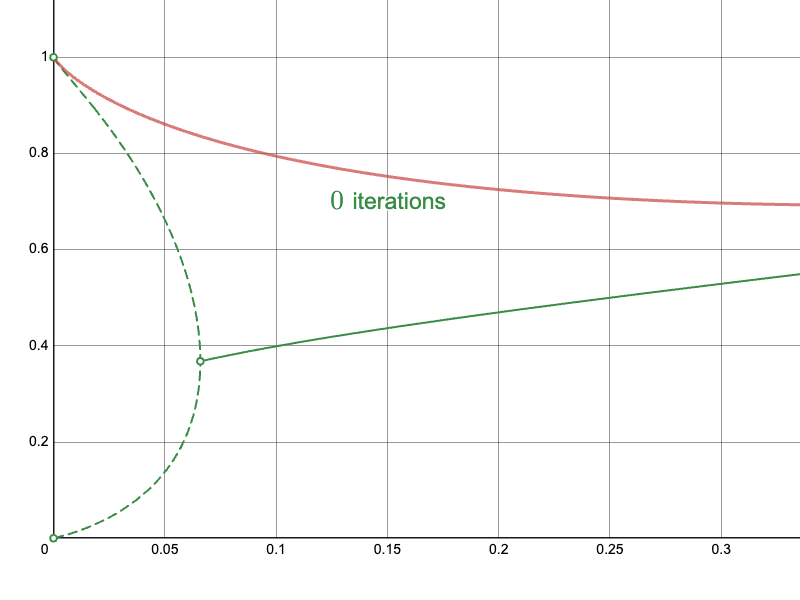
If we plot this equation, we get the following red curve. Ignore the green curve for now (we’ll talk about it shortly):

Interestingly, if we instead graph the application of two iterations:
\[x^{x^y}=y\]
Then we get the same curve, but with an additional two branches when x is small, colored above as the green curve. These two green branches correspond to the values which the naïve sequence oscillates between in the limit as the number of iterations approaches infinity. When \(x\) is larger than where the green curve exists, the sequence will converge on the red curve. Finally, to the right of the point where the red curve bends backward (to the left, where there now appear to be multiple values for the tetration for a single input), which is also the upper bound on the domain of the curve, all values will diverge to infinity.
Why do the branches only appear with the more complicated expression? If you compute the iteration only once, then in the oscillatory region, the value will flip to the other value between which the sequence is oscillating. But if you apply the iteration twice, then the value will flip twice, back to its original value. The first graph plots what is invariant under a single iteration, while the second graph plots what is invariant under two iterations.
I want to briefly also talk about the red-colored “middle” branch that lies between the two green branches. We observed before that repeatedly exponentiating \(x\) to its own power in this oscillatory region causes the value to oscillate between the two green branches. The middle branch is sort of a “ghost” solution—it satisfies the property that raising \(x\) to its values returns the same values (which is consistent with how we described the infinite tetration), but if we begin with \(x\) and repeatedly construct a larger and larger power tower, we will never reach this branch. Thus, I am not sure whether to call this a “valid solution” to the infinite tetration or not.
Deriving Key Points
Let’s establish some important points on the curve. The trivial cases are when \(x=0\) and \(x=1\). When \(x=0\), the infinite tetration oscillates between 0 and 1. This is because anything raised to the power of 0 is 1, and anything raised to the power of 1 is unaffected. So \(0^0=1\), \(0^{0^0}=0^{1}=0\), and the cycle repeats. Raising 1 to the power of itself is just 1, so the infinite tetration of 1 is 1.
Let’s find out where the curve goes from converging to diverging. The curve is vertical when \(\frac{dx}{dy}=0\). We can solve for \(x\): \[x^y=y\implies x = \sqrt[y]{y}\] And differentiate: \[\frac{dx}{dy}=-y^{\frac{1}{y}-2}(\ln(y)-1)=0\] Which is true when \(y^{\frac{1}{y}-2}=0\) and when \(\ln(y)=1\). Thus, the curve is vertical when \(y=0\) and when \(y=e\). That means the curve is vertical when \(x=0\) and \(x=\sqrt[e]{e}\). This tells us when the infinite tetration will diverge to infinity: whenever we are infinitely tetrating a number greater than \(\sqrt[e]{e}\). The largest value that can be infinitely-tetrated is \(\sqrt[e]{e}\), converging to the largest infinitely-tetrated value, \(e\).
To find when the curve transitions from oscillating to converging to a single value, we can use the Banach fixed-point theorem. The derivative of the fixed-point iteration \(f\left(y\right)=x^{y}\) is: \[f’\left(y\right)=\frac{d}{dy}\left[x^{y}\right]=x^{y}\ln\left(x\right)\] Because the basin of attraction is where the magnitude of the derivative is less than 1, the boundary of the basin is when the derivative is exactly 1 or -1. If we consider \(0 < x < 1\), then \(\ln(x)\) is strictly negative and \(x^y\) is strictly positive, meaning g’(y) is strictly negative. That means we can simply check when \(g’(y) = -1\). Thus, we are interested in the values of \(x\) such that: \[x^{y}\ln\left(x\right)=-1\implies y=\frac{\ln\left(-\frac{1}{\ln\left(x\right)}\right)}{\ln\left(x\right)}\] We also know, additionally, that \(x^{y}=y\), so: \[x^{\frac{\ln\left(-\frac{1}{\ln\left(x\right)}\right)}{\ln\left(x\right)}}=\frac{\ln\left(-\frac{1}{\ln\left(x\right)}\right)}{\ln\left(x\right)}\] \[\implies-\frac{1}{\ln(x)}=\frac{\ln\left(-\frac{1}{\ln(x)}\right)}{\ln(x)}\] \[\implies \frac{\ln\left(-\frac{1}{\ln(x)}\right)+1}{\ln(x)}=0\] \[\implies x=e^{-e}\] And \[y=\frac{\ln\left(-\frac{1}{\ln\left(e^{-e}\right)}\right)}{\ln\left(e^{-e}\right)}=\frac{1}{e}\]
Indeed, the curve is undefined on \(\left(-\infty,0\right)\), oscillates on \(\left[0,e^{-e}\right)\), converges on \(\left[e^{-e},\sqrt[e]{e}\right]\), and diverges on \(\left(\sqrt[e]{e},\infty\right)\).
What we would like to do is formulate a method that efficiently converges to all branches in order to determine what the infinite tetration converges to, what it tends toward, or what it oscillates between.
Before we move onto the next section, I want to briefly provide very precise upper and lower bounds for what an input \(x\) could be given some infinite tetration \(y\) in the convergent region. I’ve obtained these via Padé approximation:
\[\frac{5+\left(77y-40\right)y}{13+\left(\left(4y+35\right)y-10\right)y}\le x\le3\cdot\frac{399+\left(\left(279y+3721\right)y-2379\right)y}{1072-\left(133+\left(\left(89y-1709\right)y-3501\right)y\right)y}\]
If you are on a small device such as a phone, you can scroll to see the entire formula. These bounds are very accurate:

The infinite tetration curve is plotted in blue, the bounds are in orange, and the box of convergence is in green. The bounds are too accurate in the convergence box, so it is difficult to plot it. Here is only the convergence region:

While I will not use them in this blog post, feel free to use them if you work on this subject any more.
Lambert W
Our first step should be to attempt to solve for the infinite tetration, \( y \), directly. However, in order to solve for \(y\) exactly, we require the Lambert W function \(W(z)\), which can not be expressed using only elementary functions. The Lambert W function is the function that satisfies:
\[W(z) e^{W(z)} = z\]
You can get this result by rearranging \(y=x^y\) into
\[\ln\left(\frac{1}{y}\right)e^{\ln\left(\frac{1}{y}\right)}=-\ln\left(x\right)\]
And, by the definition of the Lambert W function:
\[W\left(-\ln\left(x\right)\right)e^{W\left(-\ln\left(x\right)\right)}=-\ln\left(x\right)\] \[\implies W\left(-\ln\left(x\right)\right)=\ln\left(\frac{1}{y}\right)\]
From here, we can obtain the solution in terms of the Lambert W function:
\[y=-\frac{W\left(-\ln\left(x\right)\right)}{\ln\left(x\right)}\]
Because we are left with the Lambert W function, which is irreducible, this motivates a numerical approach. The presence of that function demonstrates that it is impossible to exactly represent a formula in closed form. If our problem could be solved exactly using a finite number of elementary operations and functions, then so would the Lambert W function, which we know is not the case.
One potential technique to solve the problem is to compute the Lambert W function. We can employ an integral to compute the Lambert W function that was derived by Kalugin, Jeffrey, and Corless in 2011, giving:
\[y=-\frac{1}{\ln\left(x\right)\pi}\int_{0}^{\pi}\ln\left(1-\frac{1}{t}\ln\left(x\right)\sin\left(t\right)e^{t\cot\left(t\right)}\right)dt\]
Note that this integral gives only the center branch present in \(y=x^y\). The integrand is reasonably well-behaved and looks like this:
At the corner where \(x=\sqrt[e]{e}\) and \(t=0\), the integrand diverges to \(-\infty\). You can check this by substituting in the value for \(x\) and taking \(t\to0^{+}\) in the limit to get:
\[\lim_{t\to0^{+}}\ln\left(1-\frac{1}{t}\sin(t)e^{t\cot(t)-1}\right)\]
We’re interested in the limit of the t-dependent term:
\[\lim_{t\to0^{+}}\frac{1}{t}\sin(t)e^{t\cot(t)-1}\]
Notice that \(\sin\left(x\right)\), \(x\), and \(\cot\left(x\right)\) are all odd functions, so \({\sin\left(x\right)}/{x}\) and \(x\cot\left(x\right)\) are even, making the whole expression even. Thus, instead of only considering the right-hand limit, I will consider the limit from both sides (for simplicity, because the RH and LH limits equal each other).
Using L’Hôpital’s rule:
\[\lim_{t\to0}\frac{\sin(2t)-t}{\sin\left(t\right)}e^{t\cot(t)-1}\] \[=\lim_{t\to0}\frac{\sin(2t)-t}{\sin\left(t\right)}\cdot\lim_{t\to0}e^{t\cot(t)-1}\]
Using L’Hôpital’s rule again, the left-hand limit becomes:
\[\lim_{t\to0}\left[4 \cos (t)-3 \sec (t)\right]=1\]
Using L’Hôpital’s rule again on \(t\cot(t)={t}/{\tan\left(t\right)}\), the right-hand limit becomes:
\[\lim_{t\to0}e^{\cos^{2}\left(t\right)-1}=1\]
If you differentiate the original term \(\frac{1}{t}\sin(t)e^{t\cot(t)-1}\) twice and again solve for the limit as \(t\to0\), you will obtain a value of -1. Because the term has even symmetry and negative curvature, the term must be approaching 1 from the negative end. Thus, the limit that we were originally interested in is:
\[\lim_{t\to1^{-}}\ln\left(1-t\right)=-\infty\]
This checks out because \(t\) is not defined above 1 on the reals (we can not approach from the positive side). This shows that the integrand goes to \(-\infty\) at this point, and special measures may be useful for taking this into account when numerically approximating the integral.
It turns out that a simple substitution works nicely to tame the singularity. If we define the integrand as a function \(I\):
\[y=-\frac{1}{\ln\left(x\right)\pi}\int_{0}^{\pi}I\left(x,t\right)dt,\] \[I\left(x,t\right):=\ln\left(1-\frac{1}{t}\ln\left(x\right)\sin\left(t\right)e^{t\cot\left(t\right)}\right)\]
And make the substitution \(t=u^{2},\ dt=2u\ du\), then the integral becomes:
\[y=-\frac{1}{\ln\left(x\right)\pi}\int_{0}^{\sqrt{\pi}}2uI\left(x,u^{2}\right)du\] \[=-\frac{2}{\pi\ln(x)}\int_{0}^{\sqrt{\pi}}t\ln\left(1-\frac{1}{t^{2}}\sin\left(t^{2}\right)e^{t^{2}\cot\left(t^{2}\right)}\ln(x)\right)dt\]
This integrand looks like this:
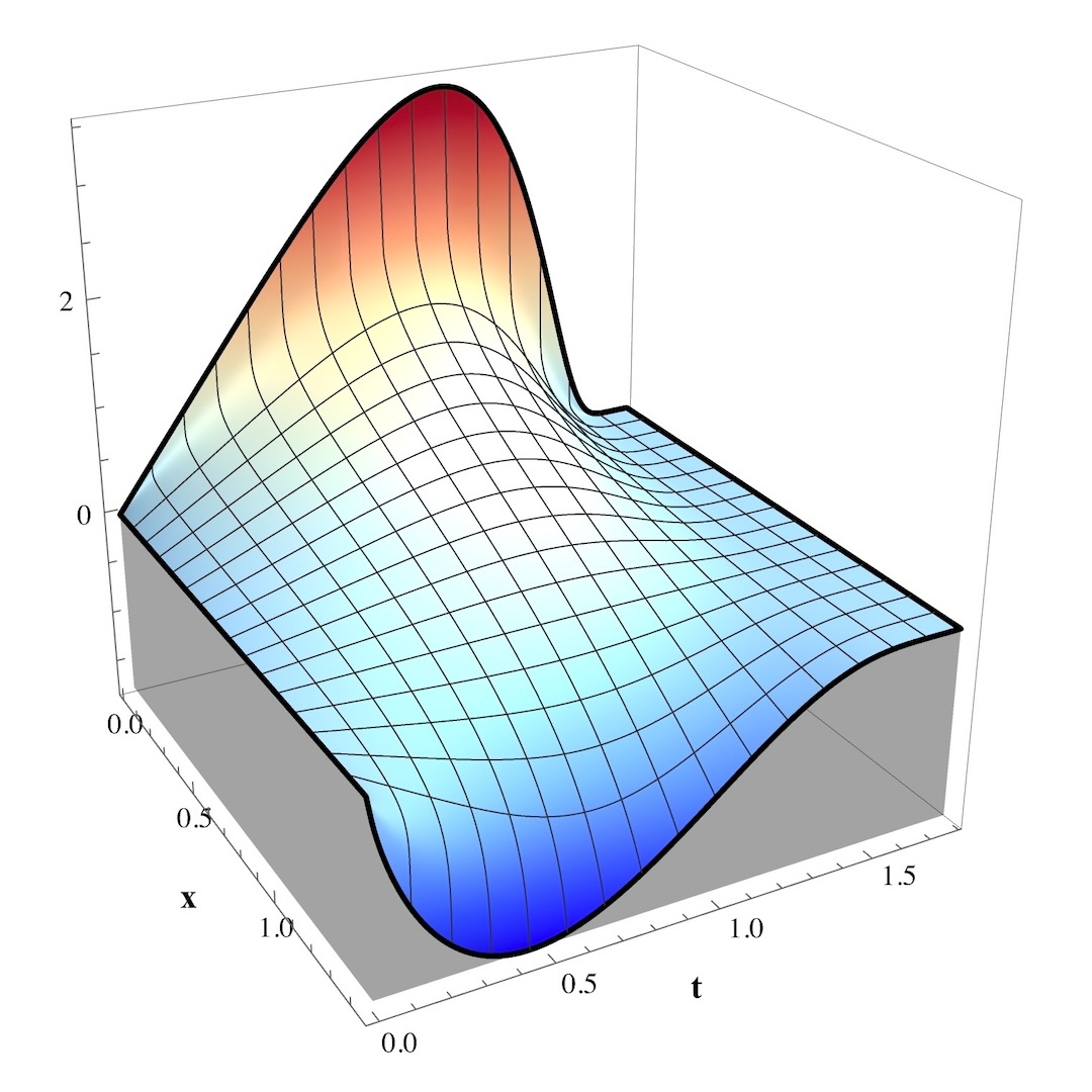
The level curves at fixed \(x\) are very nice. Note now, however, that this integrand very rapidly diverges to \(\infty\) as \(x\to0^{+}\). This is not obvious from the graph because this occurs for extremely small \(x\), but you can prove it easily; the integrand is of the form \(t\ln\left(1-f\left(t\right)\ln\left(x\right)\right)\), and \(\lim_{x\to0^{+}}\ln\left(x\right)=-\infty\). Thus you would want to use this integrand only when \(x\) is close to \(\sqrt[e]{e}\), and the other integrand otherwise.
This completes the method of solving the problem using numerical integration. In the remainder of this blog post, I will use the Newton-Raphson method (which I have discussed briefly in the previous blog post) to solve the problem.
Newton-Raphson
The general strategy that I employ for solving the problem is turning it into a root-finding problem, which we can use the Newton-Raphson method to solve provided we have a decent enough initial approximation of the curve. I will use the simpler curve \( x^y=y \) for the convergent region \(x\in\left(e^{-e},\sqrt[e]{e}\right)\) due to its minimal computational complexity. I will use the more complicated curve \(x^{x^y}=y\) for the branching region \(x\in\left(0,e^{-e}\right)\) due to its more complete structure.
We can rearrange the equations to create root-finding problems:
\[0=x^{y}-y=:g_{1}(y)\] \[0=x^{y}\ln\left(x\right)-\ln\left(y\right)=g_{2}(y)\]
I obtained the second equation by first taking the natural log of both sides to collapse the exponents. What we’ve constructed are functions \(g_{1,2}(y)\), provided some \(x\), which is 0 only when \(y\) is the infinite tetration of \(x\). For this problem, we can use the Newton-Raphson method, which I’ve briefly discussed in a previous blog post. In essence, to find \(z\) such that \(g(z)=0\), we compute the fixed-point iteration \(z\to f(z)\) where
\[z\mapsto f\left(z\right)=z-\frac{g\left(z\right)}{g’\left(z\right)}\]
And you can easily find the derivative with the quotient rule, which determines convergence via the Banach fixed-point theorem:
\[-1<f’\left(z\right)=\frac{\left|g\left(z\right)g’’\left(z\right)\right|}{g’\left(z\right)^{2}}<1\]
Using the functions which we wish to find the roots of, we can construct the Newton-Raphson iterations:
\[z\mapsto f_{1}(z)=z\cdot\frac{\ln\left(z\right)-1}{Lz-1}\] and \[z\mapsto f_{2}(z)=z\cdot\left[1+\frac{\ln\left(z\right)-L\cdot x^{z}}{L^{2}\cdot z\cdot x^{z}-1}\right]\]
Where \(L=\ln(x)\) can be precomputed. As Python code, the update procedures are:
# Initialize before iteration
L = log(x)

# Iteration for y = x^y:
z *= (log(z) - 1) / (L * z - 1)

# Iteration for y = x^x^y:
Lxz = L * x**z
z *= 1 + (log(z) - Lxz) / (z * L * Lxz - 1)
To compute the infinite tetration z of x.
Note that both methods will work in the main region where the infinite tetration converges, but only the latter method will work in the oscillatory region. In the oscillatory region, the method will tend to converge to whichever three branches the seed is closest to (but this is not always the case–check out my previous blog post on Newton Fractals). The derivative of the more complicated method is:
\[f_{2}’\left(z\right)=\frac{\left(z^{2}x^{z}L^{3}+1\right)\left(x^{z}L-\ln\left(z\right)\right)}{\left(zx^{z}L^{2}-1\right)^{2}}\]
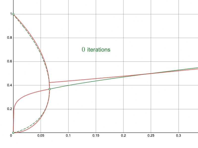
This is what the convergence basin looks like, plotted in orange, behind the fixed-point infinite tetration curve, plotted in blue:

In order to compute the tetration of a number \(x\), we must choose an initial guess \(y_0\) such that \(\left(x,y_0\right)\) is in the orange region and every point \(\left(x,y\right)\) for \(y\) between the initial guess \(y_0\) and the blue fixed-point \(y_{\infty}\) is also in the orange region.
Because we used the more “complete” curve \(x^{x^y}=y\), the fixed-point iteration \(f_{2}(y)\) can converge to any of the three branches present on the domain \(x\in\left(0,e^{-e}\right)\).
In order to use the method, however, we must provide the method with an initial guess that is close to the desired curve. We can do this by approximating the complex curve with a simpler curve.
For the main section on \(x\in\left(e^{-e},\sqrt[e]{e}\right)\), I employ a rational function approximation. If my approximation is \(R_{\beta}(x)\) where \(\beta\) are the parameters that determine a particular rational function, then my objective is to find those coefficients \(\beta\) that minimize the \(L_2\) norm of the error on the interval:
\[\min_{\beta}\int_{e^{-e}}^{\sqrt[e]{e}}\left[R_{\beta}\left(x\right)-y\left(x\right)\right]^{2}dx\]
Where \(y\) is the infinite tetration of \(x\). This approximation comes out to:
\[y\approx \frac{\left(1+2.051x\right)x-6.037}{\left(16.183-4.006x\right)x-15.134}\]
In retrospect, a minimax approximation rule would be more sensible in this context, but this approximation works great anyway. This is the approximation plotted below in red, with the actual infinite tetration curve plotted in blue, and the basin of convergence lightly shaded in orange:

I also wanted to approximate each of the branches in the oscillatory region. Sometimes, a mathematical regime is not needed to determine some “optimal” seed. Often, some educated guesswork suffices. In my case, I came up with these approximations based on the general shape of the curves that I was looking for. From top to bottom, the approximations are:
\[y_{1}\approx \frac{1}{e}\left(1+\left(e-1\right)e^{{e}/{2}}\sqrt{e^{-e}-x}\right)\] \[y_{2}\approx e^{0.15e-1}x^{0.15}\] \[y_{3}\approx \frac{1}{e}\left(1-\sqrt{1-e^{2e}x^{2}}\right)\]
These approximations look like this, plotted in red, with the actual infinite tetration curve plotted in blue, and the basin of convergence lightly shaded in orange:

Results
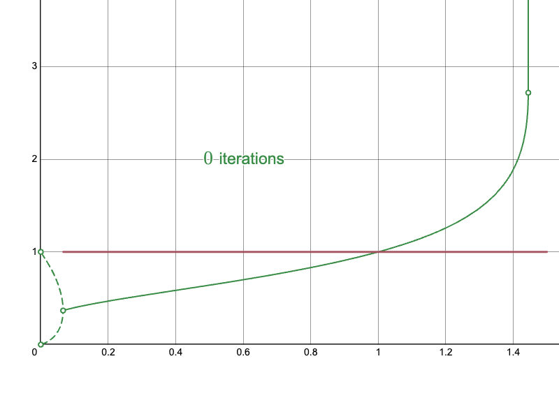
In this last part, I will present the results of the approach. Recall the naïve approach:
The derived Newton-Raphson iteration with my initial approximations converge much more quickly in difficult regions:
In particular, compare the convergence of the naïve approach near the branching point:
To the Newton-Raphson iteration:
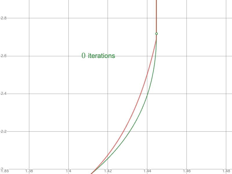
And compare the convergence of the naïve approach near the upper limit:
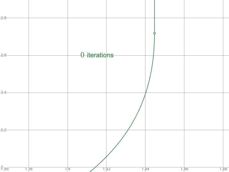
To the Newton-Raphson iteration:
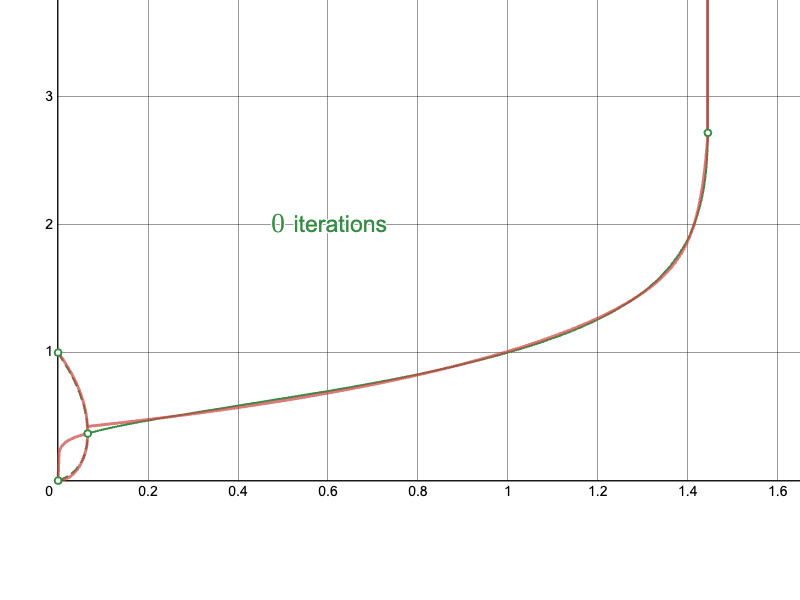
Here are the approaches overlaid for the main convergent section, with the Naïve approach in blue, the Newton-Raphson iteration in red, and the ground truth curve in green:
Here is my full implementation of the method as a Python module:
import math

BRANCH_POINT: float = math.exp(-math.e)
MAX_VALUE: float = math.exp(1 / math.e)


def compute_infinite_tetration(
    x: float,
    MAX_ITER: int = 128,
    tolerance: float = 1e-9,
    verbose: bool = False,
) -> tuple[float, ...]:
    """Computes the infinite tetration of non-negative real numbers using the Newton-Raphson method.

    Args:
        x (float): non-negative float to infinitely tetrate.
        MAX_ITER (int, optional): Number of maximum iterations allowed. Defaults to 32.
        tolerance (float, optional): Convergence tolerance. Defaults to 1e-9.

    Returns:
        tuple[float, ...]: The converged value, or the branches of the solution.
    """

    if x < 0.0:
        if math.isclose(x, -1.0):
            return (-1.0,)
        return (float("nan"),)
    elif math.isclose(x, 0.0):
        return (0.0, 1.0)
    elif math.isclose(x, 1.0):
        return (1.0,)

    elif x < BRANCH_POINT:
        z1 = (
            1 + (math.e - 1) * math.exp(math.e * 0.5) * math.sqrt(math.exp(-math.e) - x)
        ) / math.e
        z2 = math.exp(0.15 * math.e - 1) * x**0.15
        z3 = (1 - math.sqrt(1 - math.exp(2 * math.e) * x * x)) / math.e
        L = math.log(x)

        # Flags to check for convergence
        c1 = c2 = c3 = False

        # These will be L * x^z for each branch.
        Lxz1 = Lxz2 = Lxz3 = 1

        # Iterate for x^x^y = y until convergence
        for i in range(MAX_ITER):
            # Keeping track of previous z's to check for convergence
            zp1, zp2, zp3 = z1, z2, z3
            if not c1:
                Lxz1 = L * x**z1
            if not c2:
                Lxz2 = L * x**z2
            if not c3:
                Lxz3 = L * x**z3

            # These cases should NEVER occur. It is here just in case.
            if z1 < 0:
                print(f"WARNING: iteration {i + 1} encountered negative z1: {z1}")
                z1 = x**z1
            if z2 < 0:
                print(f"WARNING: iteration {i + 1} encountered negative z1: {z2}")
                z2 = x**z2
            if z3 < 0:
                print(f"WARNING: iteration {i + 1} encountered negative z1: {z3}")
                z3 = x**z3

            try:
                # Newton-Raphson iterations
                if not c1:
                    z1 *= 1 + (math.log(z1) - Lxz1) / (z1 * L * Lxz1 - 1)
                if not c2:
                    z2 *= 1 + (math.log(z2) - Lxz2) / (z2 * L * Lxz2 - 1)
                if not c3:
                    z3 *= 1 + (math.log(z3) - Lxz3) / (z3 * L * Lxz3 - 1)

            except ValueError as Err:
                print(f"Iteration {i + 1} failed with error: {Err}")
                print(f"z1 = {z1}, Lxz1 = {Lxz1}")
                print(f"z1 = {z2}, Lxz1 = {Lxz2}")
                print(f"z1 = {z3}, Lxz1 = {Lxz3}")
                return (z1, z2, z3)
            except ZeroDivisionError as Err:
                print(f"Iteration {i + 1} failed with error: {Err}")
                print(f"z1 = {z1}, Lxz1 = {Lxz1}")
                print(f"z1 = {z2}, Lxz1 = {Lxz2}")
                print(f"z1 = {z3}, Lxz1 = {Lxz3}")
                return (z1, z2, z3)

            # Check for convergence
            if not c1:
                c1 = abs(z1 - zp1) < tolerance * max(abs(z1), 1.0)
            if not c2:
                c2 = abs(z2 - zp2) < tolerance * max(abs(z2), 1.0)
            if not c3:
                c3 = abs(z3 - zp3) < tolerance * max(abs(z3), 1.0)
            if c1 and c2 and c3:
                if verbose:
                    print(f"Converged in {i} iterations.")
                return (z1, z2, z3)

        print(
            f"WARNING: iteration {i + 1} failed to converge after {MAX_ITER} iterations."
        )
        print(f"x: {x}")
        return (z1, z2, z3)

    elif x < MAX_VALUE:
        z = ((1 + 2.051 * x) * x - 6.037) / ((16.183 - 4.006 * x) * x - 15.134)
        L = math.log(x)

        # Iterate for x^y = y until convergence
        for i in range(MAX_ITER):
            zp = z  # previous z

            if z < 0:
                # This should never occur. It is here just in case.
                print(f"WARNING: iteration {i + 1} encountered negative z: {z}")
                z = x**z

            try:
                # Newton-Raphson iteration
                z *= (math.log(z) - 1) / (L * z - 1)

            except ValueError as Err:
                print(f"Iteration {i + 1} failed with ValueError: {Err}")
                print(f"z = {z}")
                return (z,)
            except ZeroDivisionError as Err:
                print(f"Iteration {i + 1} failed with ZeroDivisionError: {Err}")
                print(f"z = {z}")
                return (z,)

            if abs(z - zp) < tolerance * max(abs(z), 1.0):
                if verbose:
                    print(f"Converged in {i} iterations.")
                return (z,)

        print(
            f"WARNING: iteration {i + 1} failed to converge after {MAX_ITER} iterations."
        )
        print(f"x: {x}")
        return (z,)

    elif math.isclose(x, MAX_VALUE):
        return (math.e,)
    else:
        return (float("inf"),)
Potential improvements to my code could be to vectorize computations for the branched section of the curve using NumPy, using math.fma() to take advantage of multiplier–accumulators in modern CPUs, or just writing the code in a lower-level language like C++ or Rust instead. But the code is already blazingly fast for me, so I am satisfied with the approach.
Thanks for reading!